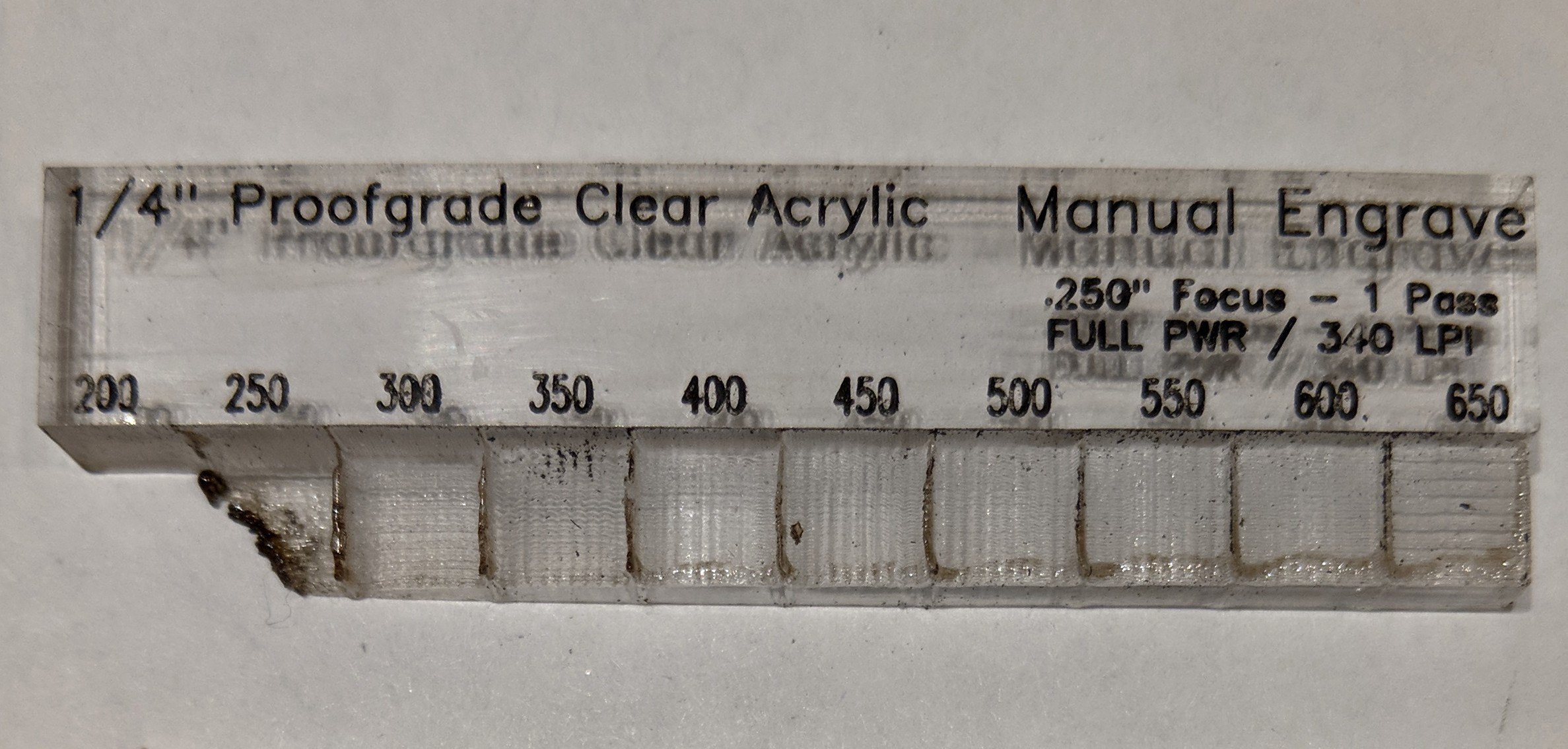
The Glowforge cloud software has an unusual way of setting the amount of laser power that hits the material. Rather than adjusting the high-voltage output to the tube, they set the voltage to its maximum, and then use a dithering algorithm to switch the laser on and off at a high speed - effectively a PWM process.
To see this in action, I ran a series of engraves, captured the stepper files, and used the Glowforge Utilities and some custom scripting to generate an image representing the laser power and firings over the engraving period.
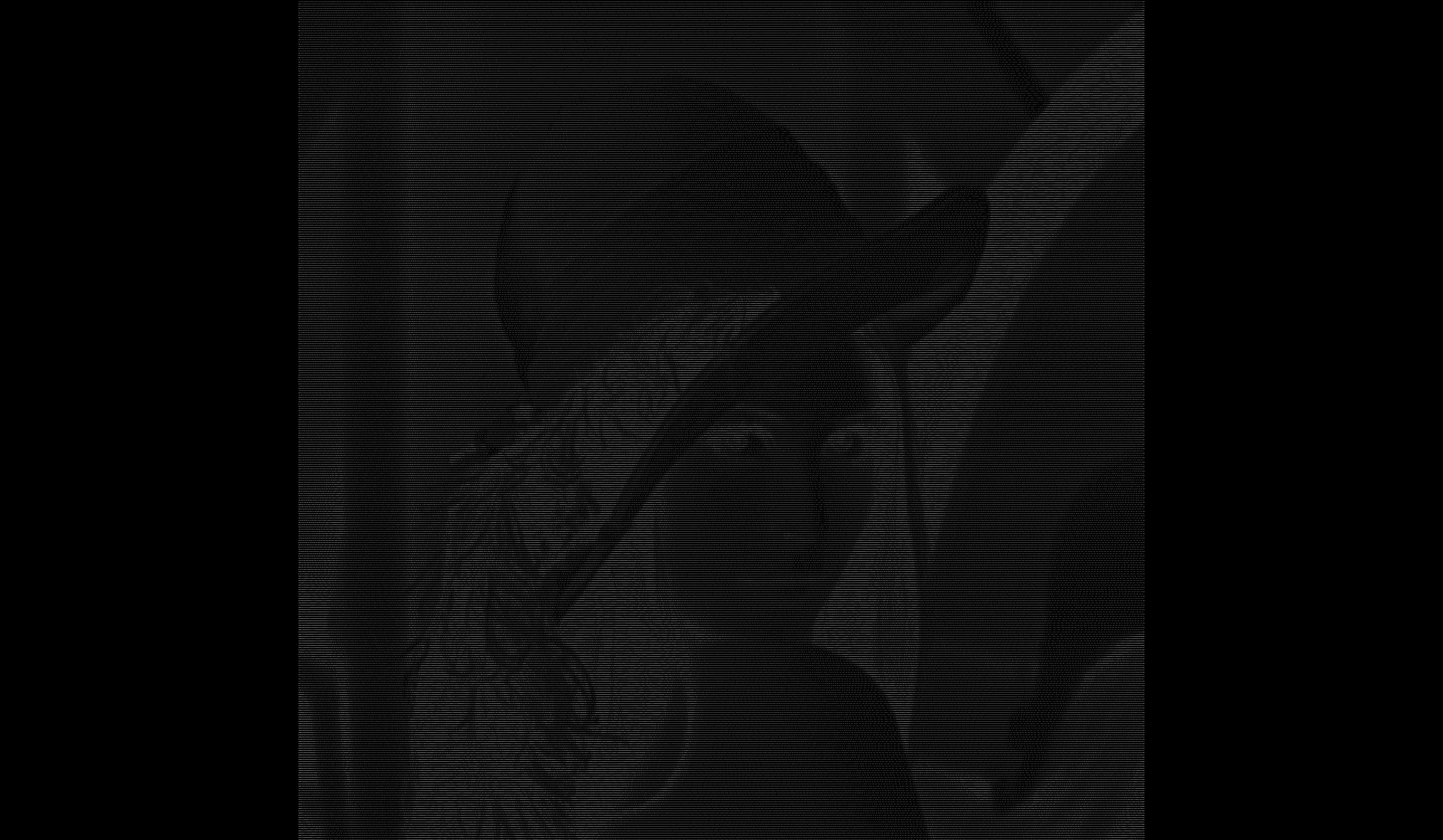
I used the following image of a solid 100% black .500" square:

( Here is the actual SVG: 500_black.zip (8.2 KB))
I set the following in the GFUI:
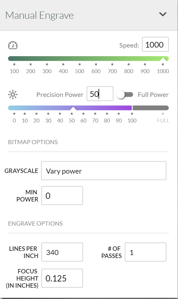
That resulted in this stepper waveform file: MAN_VP_1000_50_0_340.zip (17.4 KB)
Next, I whipped up the this quick and dirty Python script:
from GF.MOTION import motion, steps, position, laser
from PIL import Image, ImageDraw

def new_position(cur_pos, dlt):
    """
    Calculates the XYZ position by adding the delta provided
    :param cur_pos: dict in the form: {'X': x, 'Y': y, 'Z': z}
    :param dlt: dict in the form: {'X': dx, 'Y': dy, 'Z': dz}
    :return: dict in the form: {'X': x+dx, 'Y': y+dy, 'Z': z+dz}
    """
    for axis in cur_pos:
        cur_pos[axis] = cur_pos[axis] + dlt[axis]
    return cur_pos

mot = motion.Motion('MAN_VP_1000_50_0_340')

# Find the first time we go in reverse on X axis.
# It's the easiest way to find out where our test engrave has begun.
# Of course, we lose the first line, but that's OK. It does other things well.
r_pulse = mot.raw_pulse[steps.find(mot.raw_pulse, 'X', False) - 1:]

# Now we just use the rest of it for our work.
r_pulse = r_pulse[steps.find(r_pulse, 'X', True) - 1:]

# Find out how big of an array we need for our image and initialize it with zeros
extents = position.extents(r_pulse)
img = Image.new('RGB', (extents['XP'] + 1, extents['YP'] + 1))
draw = ImageDraw.Draw(img)

# Reset our position counter
pos = {'X': 0, 'Y': 0, 'Z': 0}

# Start drawing out the picture
while True:
    # Find next step in the pulse file
    step_loc = steps.find(r_pulse)
    if not step_loc:
        # No more steps, we are done
        break
    # Grab the chunk of the pulse data between now and the last step
    chunk = r_pulse[0:step_loc]
    # Remove that space from the remaining pulse data
    r_pulse = r_pulse[step_loc:]
    # Calculate the new head position
    pos = new_position(pos, position.delta(chunk))
    # Calculate how much laser power we threw down
    power = int((float(laser.on_count(chunk)) / float(step_loc)) * 255)
    # Plot the laser power data on the image at the current location
    draw.point((pos['X'], extents['YP'] - pos['Y']), fill=(power, power, power))

# We're done. Save the image.
img.save(name + '.png', 'PNG', compress_level=0, optimze=False)
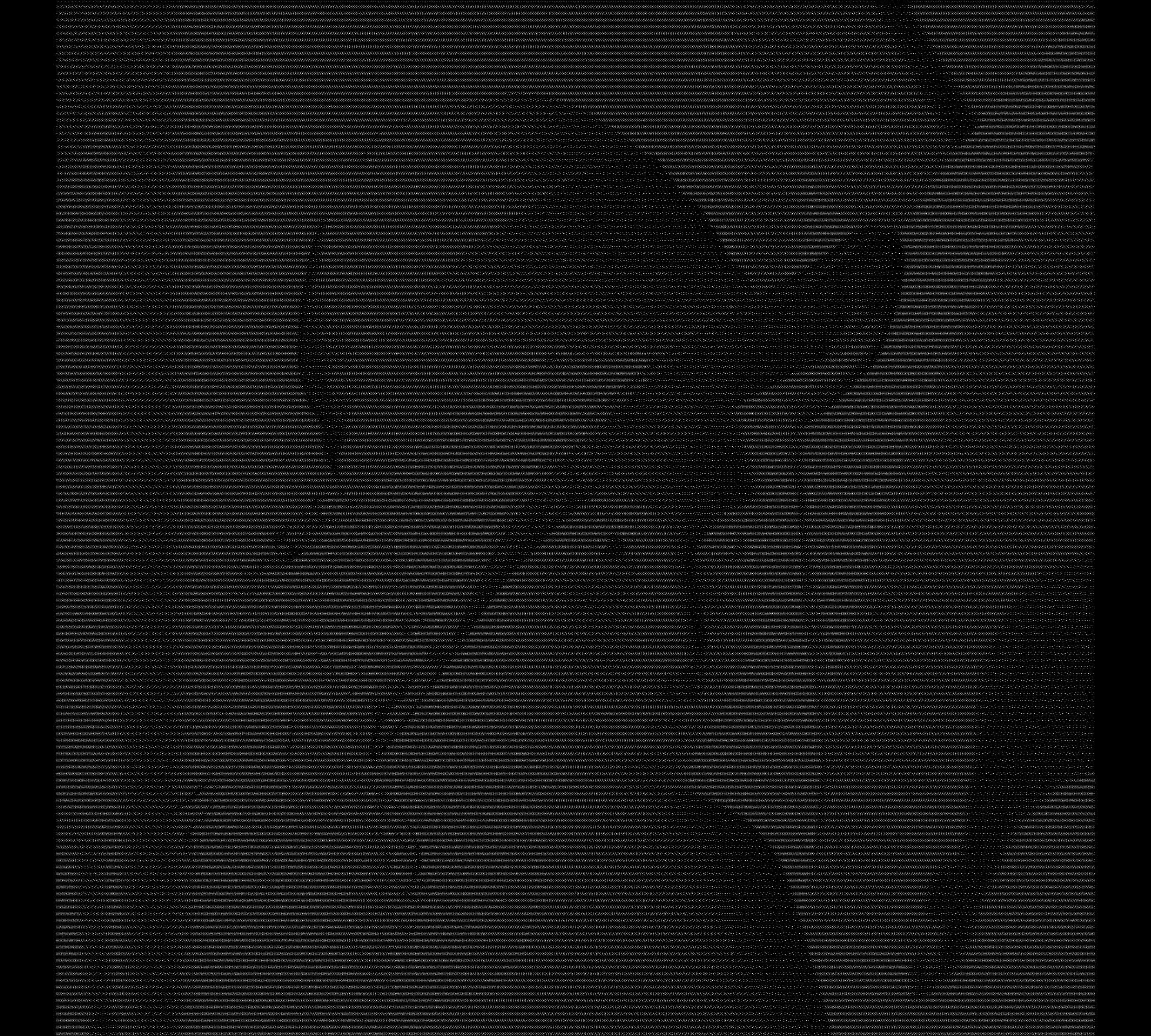
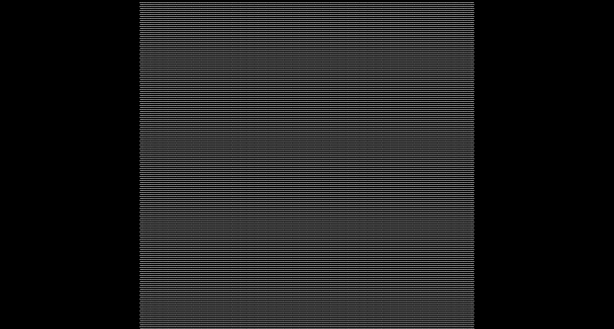
That (horribly inefficient, but effective) code spits out the following image:

You can see from the picture how a dot pattern artifact was introduced to our solid object engraving. This is where the ‘tweed’ pattern you see in solid engravings is coming from.
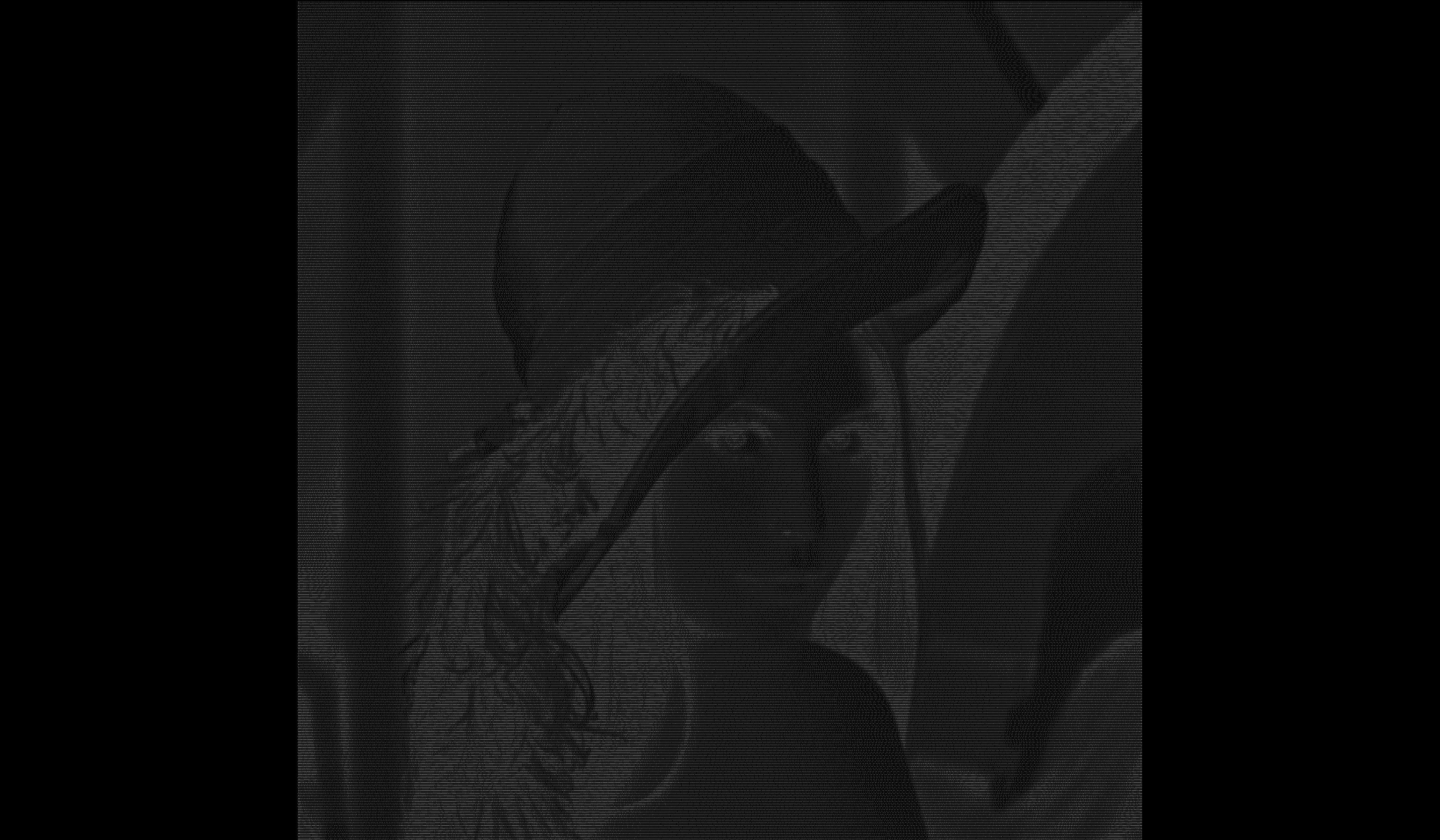
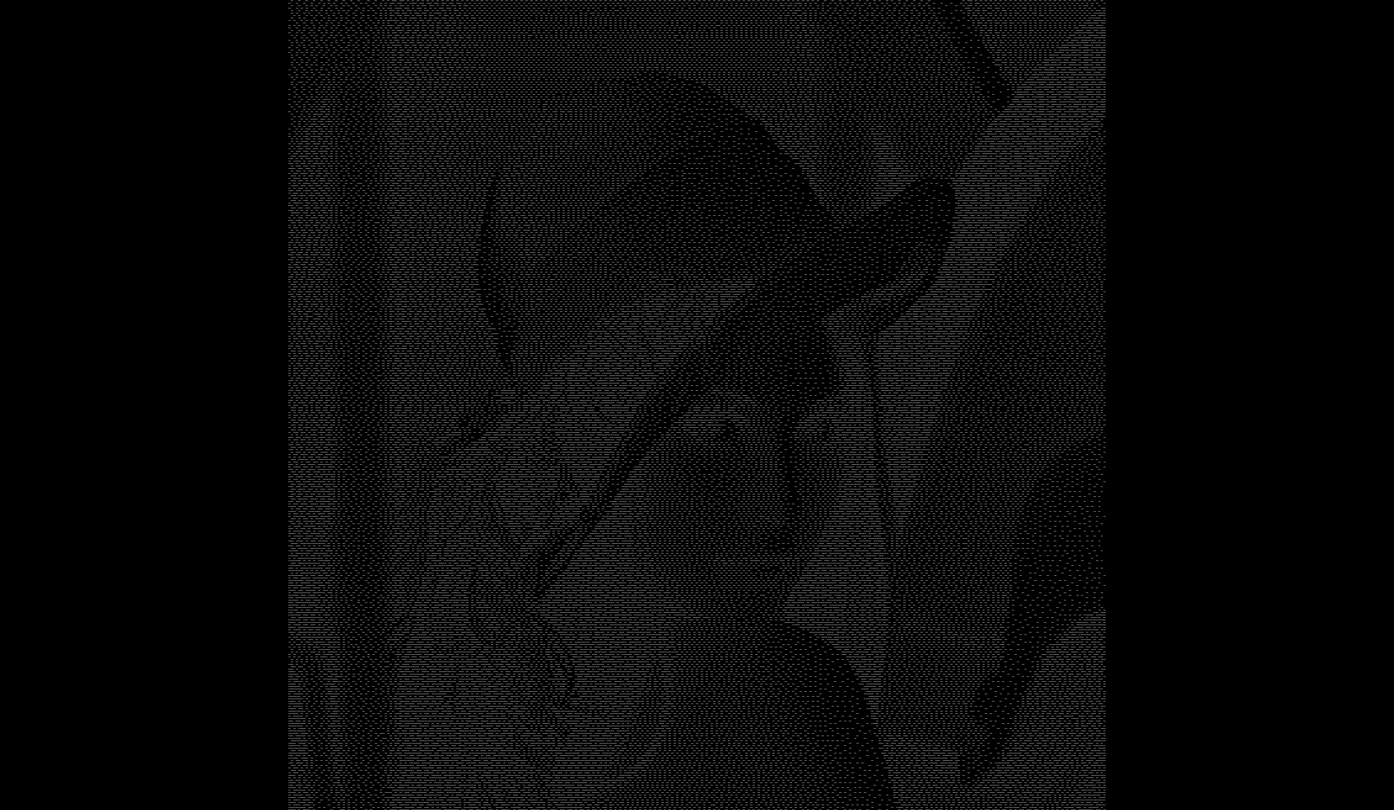
Here are results from several of my tests:
(the multiplier I use for each image may have varied in order to get a decent picture, so your mileage may vary)
Manual Engrave, 500 Speed, 10% Precision Power, 340 LPI: MAN_VP_500_10_0_340.zip (19.1 KB)

Manual Engrave, 500 Speed, 50% Precision Power, 340 LPI: MAN_VP_500_50_0_340.zip (16.4 KB)

Manual Engrave, 500 Speed, 100% Precision Power, 340 LPI: MAN_VP_500_100_0_340.zip (18.1 KB)
Manual Engrave, 1000 Speed, 10% Precision Power, 340 LPI: MAN_VP_1000_10_0_340.zip (17.0 KB)

Manual Engrave, 1000 Speed, 50% Precision Power, 340 LPI: MAN_VP_1000_50_0_340.zip (17.4 KB)
Manual Engrave, 1000 Speed, 100% Precision Power, 340 LPI: MAN_VP_1000_100_0_340.zip (17.2 KB)